Large margin nearest neighbor

Large margin nearest neighbor (LMNN)^[1] classification is a statistical machine learning algorithm for metric learning. It learns a pseudometric designed for k-nearest neighbor classification. The algorithm is based on semidefinite programming, a sub-class of convex optimization.

The goal of supervised learning (more specifically classification) is to learn a decision rule that can categorize data instances into pre-defined classes. The k-nearest neighbor rule assumes a training data set of labeled instances (i.e. the classes are known). It classifies a new data instance with the class obtained from the majority vote of the k closest (labeled) training instances. Closeness is measured with a pre-defined metric. Large margin nearest neighbors is an algorithm that learns this global (pseudo-)metric in a supervised fashion to improve the classification accuracy of the k-nearest neighbor rule.

Setup

The main intuition behind LMNN is to learn a pseudometric under which all data instances in the training set are surrounded by at least k instances that share the same class label. If this is achieved, the leave-one-out error (a special case of cross validation) is minimized. Let the training data consist of a data set $D=\{({\vec x}_{1},y_{1}),\dots ,({\vec x}_{n},y_{n})\}\subset R^{d}\times C$ , where the set of possible class categories is $C=\{1,\dots ,c\}$ .

The algorithm learns a pseudometric of the type

d({\vec x}_{i},{\vec x}_{j})=({\vec x}_{i}-{\vec x}_{j})^{\top }{\mathbf {M}}({\vec x}_{i}-{\vec x}_{j})

For $d(\cdot ,\cdot )$ to be well defined, the matrix $\mathbf {M}$ needs to be positive semi-definite. The Euclidean metric is a special case, where $\mathbf {M}$ is the identity matrix. This generalization is often (falsely) referred to as Mahalanobis metric.

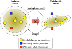
Figure 1 illustrates the effect of the metric under varying $\mathbf {M}$ . The two circles show the set of points with equal distance to the center ${\vec {x}}_{i}$ . In the Euclidean case this set is a circle, whereas under the modified (Mahalanobis) metric it becomes an ellipsoid.

Figure 1: Schematic illustration of LMNN.

The algorithm distinguishes between two types of special data points: target neighbors and impostors.

Target neighbors

Target neighbors are selected before learning. Each instance ${\vec {x}}_{i}$ has exactly $k$ different target neighbors within $D$ , which all share the same class label $y_{i}$ . The target neighbors are the data points that should become nearest neighbors under the learned metric. Let us denote the set of target neighbors for a data point ${\vec {x}}_{i}$ as $N_{i}$ .

Impostors

An impostor of a data point ${\vec {x}}_{i}$ is another data point ${\vec x}_{j}$ with a different class label (i.e. $y_{i}\neq y_{j}$ ) which is one of the nearest neighbors of ${\vec {x}}_{i}$ . During learning the algorithm tries to minimize the number of impostors for all data instances in the training set.

Algorithm

Large margin nearest neighbors optimizes the matrix $\mathbf {M}$ with the help of semidefinite programming. The objective is twofold: For every data point ${\vec {x}}_{i}$ , the target neighbors should be close and the impostors should be far away. Figure 1 shows the effect of such an optimization on an illustrative example. The learned metric causes the input vector ${\vec {x}}_{i}$ to be surrounded by training instances of the same class. If it was a test point, it would be classified correctly under the $k=3$ nearest neighbor rule.

The first optimization goal is achieved by minimizing the average distance between instances and their target neighbors

\sum _{{i,j\in N_{i}}}d({\vec x}_{i},{\vec x}_{j})

The second goal is achieved by constraining impostors ${\vec x}_{l}$ to be one unit further away than target neighbors ${\vec x}_{j}$ (and therefore pushing them out of the local neighborhood of ${\vec {x}}_{i}$ ). The resulting inequality constraint can be stated as:

\forall _{{i,j\in N_{i},l,y_{l}\neq y_{i}}}d({\vec x}_{i},{\vec x}_{j})+1\leq d({\vec x}_{i},{\vec x}_{l})

The margin of exactly one unit fixes the scale of the matrix $M$ . Any alternative choice $c>0$ would result in a rescaling of $M$ by a factor of $1/c$ .

The final optimization problem becomes:

\min _{{{\mathbf {M}}}}\sum _{{i,j\in N_{i}}}d({\vec x}_{i},{\vec x}_{j})+\sum _{{i,j,l}}\xi _{{ijl}}

\forall _{{i,j\in N_{i},l,y_{l}\neq y_{i}}}

d({\vec x}_{i},{\vec x}_{j})+1\leq d({\vec x}_{i},{\vec x}_{l})+\xi _{{ijl}}

\xi _{{ijl}}\geq 0

{\mathbf {M}}\succeq 0

Here the slack variables $\xi _{{ijl}}$ absorb the amount of violations of the impostor constraints. Their overall sum is minimized. The last constraint ensures that $\mathbf {M}$ is positive semi-definite. The optimization problem is an instance of semidefinite programming (SDP). Although SDPs tend to suffer from high computational complexity, this particular SDP instance can be solved very efficiently due to the underlying geometric properties of the problem. In particular, most impostor constraints are naturally satisfied and do not need to be enforced during runtime. A particularly well suited solver technique is the working set method, which keeps a small set of constraints that are actively enforced and monitors the remaining (likely satisfied) constraints only occasionally to ensure correctness.

Extensions and efficient solvers

LMNN was extended to multiple local metrics in the 2008 paper.^[2] This extension significantly improves the classification error, but involves a more expensive optimization problem. In their 2009 publication in the Journal of Machine Learning Research,^[3] Weinberger and Saul derive an efficient solver for the semi-definite program. It can learn a metric for the MNIST handwritten digit data set in several hours, involving billions of pairwise constraints. An open source Matlab implementation is freely available at the authors web page.

Kumal et al.^[4] extended the algorithm to incorporate local invariances to multivariate polynomial transformations and improved regularization.

References

↑ Weinberger, K. Q.; Blitzer J. C.; Saul L. K. (2006). "Distance Metric Learning for Large Margin Nearest Neighbor Classification,". Advances in Neural Information Processing Systems. 18: 1473–1480.
↑ Weinberger, K. Q.; Saul L. K. (2008). "Fast solvers and efficient implementations for distance metric learning" (PDF). Proceedings of International Conference on Machine Learning: 1160–1167.
↑ Weinberger, K. Q.; Saul L. K. (2009). "Distance Metric Learning for Large Margin Classification" (PDF). Journal of Machine Learning Research. 10: 207–244.
↑ Kumar, M.P.; Torr P.H.S.; Zisserman A. (2007). "An invariant large margin nearest neighbour classifier". IEEE 11th International Conference on Computer Vision (ICCV), 2007: 1–8.

External links

This article is issued from Wikipedia - version of the 11/28/2016. The text is available under the Creative Commons Attribution/Share Alike but additional terms may apply for the media files.