Mixture distribution
In probability and statistics, a mixture distribution is the probability distribution of a random variable that is derived from a collection of other random variables as follows: first, a random variable is selected by chance from the collection according to given probabilities of selection, and then the value of the selected random variable is realized. The underlying random variables may be random real numbers, or they may be random vectors (each having the same dimension), in which case the mixture distribution is a multivariate distribution.
In cases where each of the underlying random variables is continuous, the outcome variable will also be continuous and its probability density function is sometimes referred to as a mixture density. The cumulative distribution function (and the probability density function if it exists) can be expressed as a convex combination (i.e. a weighted sum, with non-negative weights that sum to 1) of other distribution functions and density functions. The individual distributions that are combined to form the mixture distribution are called the mixture components, and the probabilities (or weights) associated with each component are called the mixture weights. The number of components in mixture distribution is often restricted to being finite, although in some cases the components may be countably infinite. More general cases (i.e. an uncountable set of component distributions), as well as the countable case, are treated under the title of compound distributions.
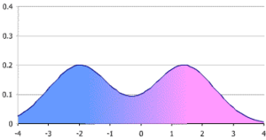
A distinction needs to be made between a random variable whose distribution function or density is the sum of a set of components (i.e. a mixture distribution) and a random variable whose value is the sum of the values of two or more underlying random variables, in which case the distribution is given by the convolution operator. As an example, the sum of two jointly normally distributed random variables, each with different means, will still have a normal distribution. On the other hand, a mixture density created as a mixture of two normal distributions with different means will have two peaks provided that the two means are far enough apart, showing that this distribution is radically different from a normal distribution.
Mixture distributions arise in many contexts in the literature and arise naturally where a statistical population contains two or more subpopulations. They are also sometimes used as a means of representing non-normal distributions. Data analysis concerning statistical models involving mixture distributions is discussed under the title of mixture models, while the present article concentrates on simple probabilistic and statistical properties of mixture distributions and how these relate to properties of the underlying distributions.
Finite and countable mixtures

Given a finite set of probability density functions p1(x), …, pn(x), or corresponding cumulative distribution functions P1(x), …, Pn(x) and weights w1, …, wn such that wi ≥ 0 and ∑wi = 1, the mixture distribution can be represented by writing either the density, f, or the distribution function, F, as a sum (which in both cases is a convex combination):
This type of mixture, being a finite sum, is called a finite mixture, and in applications, an unqualified reference to a "mixture density" usually means a finite mixture. The case of a countably infinite set of components is covered formally by allowing .
Uncountable mixtures
Where the set of component distributions is uncountable, the result is often called a compound probability distribution. The construction of such distributions has a formal similarity to that of mixture distributions, with either infinite summations or integrals replacing the finite summations used for finite mixtures.
Consider a probability density function p(x;a) for a variable x, parameterized by a. That is, for each value of a in some set A, p(x;a) is a probability density function with respect to x. Given a probability density function w (meaning that w is nonnegative and integrates to 1), the function
is again a probability density function for x. A similar integral can be written for the cumulative distribution function. Note that the formulae here reduce to the case of a finite or infinite mixture if the density w is allowed to be a generalized function representing the "derivative" of the cumulative distribution function of a discrete distribution.
Mixtures of parametric families
The mixture components are often not arbitrary probability distributions, but instead are members of a parametric family (such as normal distributions), with different values for a parameter or parameters. In such cases, assuming that it exists, the density can be written in the form of a sum as:
for one parameter, or
for two parameters, and so forth.
Properties
Convexity
A general linear combination of probability density functions is not necessarily a probability density, since it may be negative or it may integrate to something other than 1. However, a convex combination of probability density functions preserves both of these properties (non-negativity and integrating to 1), and thus mixture densities are themselves probability density functions.
Moments
Let X1, ..., Xn denote random variables from the n component distributions, and let X denote a random variable from the mixture distribution. Then, for any function H(·) for which exists, and assuming that the component densities pi(x) exist,
It is a trivial matter to note that the jth moment about zero (i.e. choosing H(x) = xj) is simply a weighted average of the jth moments of the components. Moments about the mean H(x) = (x − μ)j involve a binomial expansion:[1]
where μi denotes the mean of the ith component.
In case of a mixture of one-dimensional distributions with weights wi, means μi and variances σi2, the total mean and variance will be:
These relations highlight the potential of mixture distributions to display non-trivial higher-order moments such as skewness and kurtosis (fat tails) and multi-modality, even in the absence of such features within the components themselves. Marron and Wand (1992) give an illustrative account of the flexibility of this framework.[2]
Modes
The question of multimodality is simple for some cases, such as mixtures of exponential distributions: all such mixtures are unimodal.[3] However, for the case of mixtures of normal distributions, it is a complex one. Conditions for the number of modes in a multivariate normal mixture are explored by Ray and Lindsay[4] extending the earlier work on univariate [5][6] and multivariate distributions (Carreira-Perpinan and Williams, 2003[7]).
Here the problem of evaluation of the modes of a n component mixture in a D dimensional space is reduced to identification of critical points (local minima, maxima and saddle points) on a manifold referred to as the ridgeline surface, which is the image of the ridgeline function
where α belongs to the n − 1 dimensional unit simplex and Σi ∈ RD × D, μi ∈ RD correspond to the covariance and mean of the ith component. Ray and Lindsay consider the case in which n − 1 < D showing a one-to-one correspondence of modes of the mixture and those on the elevation function h(α) = q(x*(α)) thus one may identify the modes by solving with respect to α and determining the value x*(α).
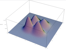
Using graphical tools, the potential multi-modality of n = {2, 3} mixtures is demonstrated; in particular it is shown that the number of modes may exceed n and that the modes may not be coincident with the component means. For two components they develop a graphical tool for analysis by instead solving the aforementioned differential with respect to w1 and expressing the solutions as a function Π(α), α ∈ [0, 1] so that the number and location of modes for a given value of w1 corresponds to the number of intersections of the graph on the line Π(α) = w1. This in turn can be related to the number of oscillations of the graph and therefore to solutions of leading to an explicit solution for a two component homoscedastic mixture given by
where dM(μ1, μ2, Σ) = (μ2 − μ1)TΣ−1(μ2 − μ1) is the Mahalanobis distance.
Since the above is quadratic it follows that in this instance there are at most two modes irrespective of the dimension or the weights.
Examples
Simple examples can be given by a mixture of two normal distributions.
Given an equal (50/50) mixture of two normal distributions with the same standard deviation and different means (homoscedastic), the overall distribution will exhibit low kurtosis relative to a single normal distribution – the means of the subpopulations fall on the shoulders of the overall distribution. If sufficiently separated, namely by twice the (common) standard deviation, so these form a bimodal distribution, otherwise it simply has a wide peak.[8] The variation of the overall population will also be greater than the variation of the two subpopulations (due to spread from different means), and thus exhibits overdispersion relative to a normal distribution with fixed variation though it will not be overdispersed relative to a normal distribution with variation equal to variation of the overall population.
Alternatively, given two subpopulations with the same mean and different standard deviations, the overall population will exhibit high kurtosis, with a sharper peak and heavier tails (and correspondingly shallower shoulders) than a single distribution.
-

Univariate mixture distribution, showing bimodal distribution
-

Multivariate mixture distribution, showing four modes
Applications
Mixture densities are complicated densities expressible in terms of simpler densities (the mixture components), and are used both because they provide a good model for certain data sets (where different subsets of the data exhibit different characteristics and can best be modeled separately), and because they can be more mathematically tractable, because the individual mixture components can be more easily studied than the overall mixture density.
Mixture densities can be used to model a statistical population with subpopulations, where the mixture components are the densities on the subpopulations, and the weights are the proportions of each subpopulation in the overall population.
Mixture densities can also be used to model experimental error or contamination – one assumes that most of the samples measure the desired phenomenon,
Parametric statistics that assume no error often fail on such mixture densities – for example, statistics that assume normality often fail disastrously in the presence of even a few outliers – and instead one uses robust statistics.
In meta-analysis of separate studies, study heterogeneity causes distribution of results to be a mixture distribution, and leads to overdispersion of results relative to predicted error. For example, in a statistical survey, the margin of error (determined by sample size) predicts the sampling error and hence dispersion of results on repeated surveys. The presence of study heterogeneity (studies have different sampling bias) increases the dispersion relative to the margin of error.
See also
- Convex combination
- Expectation-maximization algorithm
- Fat tail
- Not to be confused with: List of convolutions of probability distributions
- Product distribution
Mixture
Hierarchical models
Notes
- ↑ Frühwirth-Schnatter (2006, Ch.1.2.4)
- ↑ Marron, J. S.; Wand, M. P. (1992). "Exact Mean Integrated Squared Error". The Annals of Statistics. 20 (2): 712–736., http://projecteuclid.org/euclid.aos/1176348653
- ↑ Frühwirth-Schnatter (2006, Ch.1)
- ↑ Ray, R.; Lindsay, B. (2005), "The topography of multivariate normal mixtures", The Annals of Statistics, 33 (5): 2042–2065
- ↑ Robertson CA, Fryer JG (1969) Some descriptive properties of normal mixtures. Skand Aktuarietidskr 137–146
- ↑ Behboodian J (1970) On the modes of a mixture of two normal distributions. Technometrics 12: 131–139
- ↑ http://faculty2.ucmerced.edu/mcarreira-perpinan/papers/EDI-INF-RR-0159.pdf
- ↑ Schilling, Mark F.; Watkins, Ann E.; Watkins, William (2002). "Is Human Height Bimodal?". The American Statistician. 56 (3): 223–229. doi:10.1198/00031300265.
References
- Frühwirth-Schnatter, Sylvia (2006), Finite Mixture and Markov Switching Models, Springer, ISBN 978-1-4419-2194-9
- Lindsay, Bruce G. (1995), Mixture models: theory, geometry and applications, NSF-CBMS Regional Conference Series in Probability and Statistics, 5, Hayward, CA, USA: Institute of Mathematical Statistics, ISBN 0-940600-32-3