Regularization perspectives on support vector machines

Regularization perspectives on support vector machines provide a way of interpreting support vector machines (SVMs) in the context of other machine learning algorithms. SVM algorithms categorize multidimensional data, with the goal of fitting the training set data well, but also avoiding overfitting, so that the solution generalizes to new data points. Regularization algorithms also aim to fit training set data and avoid overfitting. They do this by choosing a fitting function that has low error on the training set, but also is not too complicated, where complicated functions are functions with high norms in some function space. Specifically, Tikhonov regularization algorithms choose a function that minimize the sum of training set error plus the function's norm. The training set error can be calculated with different loss functions. For example, regularized least squares is a special case of Tikhonov regularization using the squared error loss as the loss function.^[1]

Regularization perspectives on support vector machines interpret SVM as a special case Tikhonov regularization, specifically Tikhonov regularization with the hinge loss for a loss function. This provides a theoretical framework with which to analyze SVM algorithms and compare them to other algorithms with the same goals: to generalize without overfitting. SVM was first proposed in 1995 by Corinna Cortes and Vladimir Vapnik, and framed geometrically as a method for finding hyperplanes that can separate multidimensional data into two categories.^[2] This traditional geometric interpretation of SVMs provides useful intuition about how SVMs work, but is difficult to relate to other machine learning techniques for avoiding overfitting like regularization, early stopping, sparsity and Bayesian inference. However, once it was discovered that SVM is also a special case of Tikhonov regularization, regularization perspectives on SVM provided the theory necessary to fit SVM within a broader class of algorithms.^[1]^[3]^[4] This has enabled detailed comparisons between SVM and other forms of Tikhonov regularization, and theoretical grounding for why it is beneficial to use SVM's loss function, the hinge loss.^[5]

Theoretical background

In the statistical learning theory framework, an algorithm is a strategy for choosing a function $f:{\mathbf X}\to {\mathbf Y}$ given a training set $S=\{(x_{1},y_{1}),\ldots ,(x_{n},y_{n})\}$ of inputs, $x_{i}$ , and their labels, $y_{i}$ (the labels are usually $\pm 1$ ). Regularization strategies avoid overfitting by choosing a function that fits the data, but is not too complex. Specifically:

$f={\text{arg}}\min _{{f\in {\mathcal {H}}}}\left\{{\frac {1}{n}}\sum _{{i=1}}^{n}V(y_{i},f(x_{i}))+\lambda ||f||_{{\mathcal {H}}}^{2}\right\}$ ,

where ${\mathcal {H}}$ is a hypothesis space^[6] of functions, $V:{\mathbf Y}\times {\mathbf Y}\to {\mathbb R}$ is the loss function, $||\cdot ||_{{\mathcal H}}$ is a norm on the hypothesis space of functions, and $\lambda \in {\mathbb R}$ is the regularization parameter.^[7]

When ${\mathcal {H}}$ is a reproducing kernel Hilbert space, there exists a kernel function $K:{\mathbf X}\times {\mathbf X}\to {\mathbb R}$ that can be written as an $n\times n$ symmetric positive definite matrix ${\mathbf K}$ . By the representer theorem,^[8] $f(x_{i})=\sum _{{f=1}}^{n}c_{j}{\mathbf K}_{{ij}}$ , and $||f||_{{{\mathcal H}}}^{2}=\langle f,f\rangle _{{\mathcal H}}=\sum _{{i=1}}^{n}\sum _{{j=1}}^{n}c_{i}c_{j}K(x_{i},x_{j})=c^{T}{\mathbf K}c$

Special properties of the hinge loss

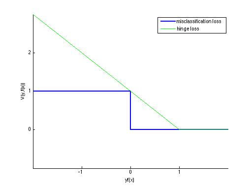
The simplest and most intuitive loss function for categorization is the misclassification loss, or 0-1 loss, which is 0 if $f(x_{i})=y_{i}$ and 1 if $f(x_{i})\neq y_{i}$ , i.e. the Heaviside step function on $-y_{i}f(x_{i})$ . However, this loss function is not convex, which makes the regularization problem very difficult to minimize computationally. Therefore, we look for convex substitutes for the 0-1 loss. The hinge loss, $V(y_{i},f(x_{i}))=(1-yf(x))_{+}$ where $(s)_{+}=max(s,0)$ , provides such a convex relaxation. In fact, the hinge loss is the tightest convex upper bound to the 0-1 misclassification loss function,^[4] and with infinite data returns the Bayes optimal solution:^[5]^[9]

$f_{b}(x)=\left\{{\begin{matrix}1&p(1|x)>p(-1|x)\\-1&p(1|x)<p(-1|x)\end{matrix}}\right.$

Derivation

The Tikhonov regularization problem can be shown to be equivalent to traditional formulations of SVM by expressing it in terms of the hinge loss.^[10] With the hinge loss,

$V(y_{i},f(x_{i}))=(1-yf(x))_{+}$

where $(s)_{+}=max(s,0)$ , the regularization problem becomes

$f={\text{arg}}\min _{{f\in {\mathcal {H}}}}\left\{{\frac {1}{n}}\sum _{{i=1}}^{n}(1-yf(x))_{+}+\lambda ||f||_{{\mathcal {H}}}^{2}\right\}$ .

Multiplying by $1/(2\lambda )$ yields

$f={\text{arg}}\min _{{f\in {\mathcal {H}}}}\left\{C\sum _{{i=1}}^{n}(1-yf(x))_{+}+{\frac {1}{2}}||f||_{{\mathcal {H}}}^{2}\right\}$ ,

with $C=1/(2\lambda n)$ , which is equivalent to the standard SVM minimization problem.

Notes and references

1 2 Rosasco, Lorenzo. "Regularized Least-Squares and Support Vector Machines" (PDF).
↑ Cortes, Corinna; Vladimir Vapnik (1995). "Suppor-Vector Networks". Machine Learning. 20: 273–297. doi:10.1007/BF00994018.
↑ Rifkin, Ryan (2002). Everything Old is New Again: A Fresh Look at Historical Approaches in Machine Learning (PDF). MIT (PhD thesis).
1 2 Lee, Yoonkyung; Wahba, Grace (2012). "Multicategory Support Vector Machines". Journal of the American Statistical Association. 99 (465): 67–81. doi:10.1198/016214504000000098.
1 2 Rosasco L, De Vito E, Caponnetto A, Piana M, Verri A (May 2004). "Are Loss Functions All the Same". Neural Computation. 5. 16: 1063–1076. doi:10.1162/089976604773135104. PMID 15070510.
↑ A hypothesis space is the set of functions used to model the data in a machine learning problem. Each function corresponds to a hypothesis about the structure of the data. Typically the functions in a hypothesis space form a Hilbert space of functions with norm formed from the loss function.
↑ For insight on choosing the parameter, see, e.g., Wahba, Grace; Yonghua Wang (1990). "When is the optimal regularization parameter insensitive to the choice of the loss function". Communications in Statistics - Theory and Methods. 19 (5): 1685–1700. doi:10.1080/03610929008830285.
↑ See Scholkopf, Bernhard; Ralf Herbrich; Alex Smola (2001). "A Generalized Representer Theorem". Computational Learning Theory: Lecture Notes in Computer Science. 2111: 416–426. doi:10.1007/3-540-44581-1_27.
↑ Lin, Yi (July 2002). "Support Vector Machines and the Bayes Rule in Classification" (PDF). Data Mining and Knowledge Discovery. 6 (3): 259–275. doi:10.1023/A:1015469627679.
↑ For a detailed derivation, see Rifkin, Ryan (2002). Everything Old is New Again: A Fresh Look at Historical Approaches in Machine Learning (PDF). MIT (PhD thesis).

Evgeniou, Theodoros; Massimiliano Pontil; Tomaso Poggio (2000). "Regularization Networks and Support Vector Machines" (PDF). Advances in Computational Mathematics. 13 (1): 1–50. doi:10.1023/A:1018946025316.
Joachims, Thorsten. "SVMlight".
Vapnik, Vladimir (1999). The Nature of Statistical Learning Theory. New York: Springer-Verlag. ISBN 0-387-98780-0.

This article is issued from Wikipedia - version of the 11/18/2016. The text is available under the Creative Commons Attribution/Share Alike but additional terms may apply for the media files.